
Structured Data and training dataset for GIS/attribute data: vegetation indexes, clustering analysis, statistics data for detection of statistically significant clusters of changes to identification of drying of tree leaves
Carrying out assessment of the territory of the forest area #1 and #2 using the combination and study of GIS/attribute data on EO Copernicus, which include the following results:
1. Perform remote sensing by used to three vegetation indexes; NDVI, NDWI and SAVI. (EO Copernicus and ESA SNAP).
2. Carrying out clustering analysis with classification by zones according to clusters/classes to obtain statistics data (ESA SNAP).
3. Transferring statistics data to GIS/attribute data (Map Info/Arc Gis online).
4. Analyses GIS/attribute data by GIS Mapping Software and/or Statistical software (ESA SNAP or IBM SPSS Statistics).
4. Analyses GIS/attribute data by GIS Mapping Software and/or Statistical software (ESA SNAP or IBM SPSS Statistics)
GIS/attribute data analysis using GIS mapping software and statistical software as IBM SPSS Statistics with results by K-Nearest Neighbors (KNN).
The KNN algorithm assumes that similar things exist nearby. In other words, similar things are next to each other.
An image that shows how similar data points are usually close to each other. Notice in the image above that most of the time similar data points are close to each other.
The KNN algorithm assumes that similar things exist nearby. In other words, similar things are next to each other.
An image that shows how similar data points are usually close to each other. Notice in the image above that most of the time similar data points are close to each other.
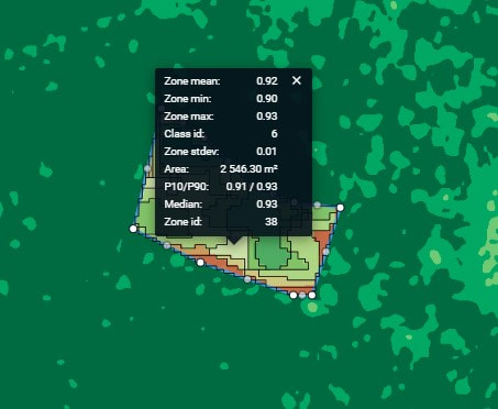
Figure 1. Presentation of statics data for zone 38, which is included with 6 class of clusters for NDVI.
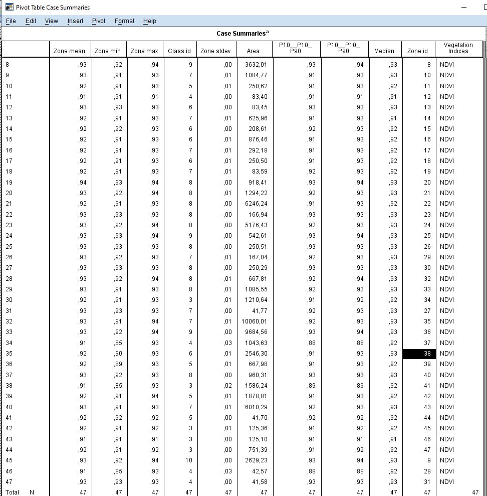
Figure 2. Presentation of the table #1 with statics data for 47 zones of forest area #1 after NDVI clustering and classification. Statics data for zone 38 represented in row 38 (#35) black colour from IBM SPSS Statistics.
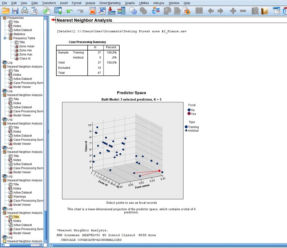
Figure 3. Presentation of the Predictor Space statistics data: zone mean, zone max, zone min and zone area from the table with statics data for 47 zones of forest area #1 (NDVI) from IBM SPSS Statistic.
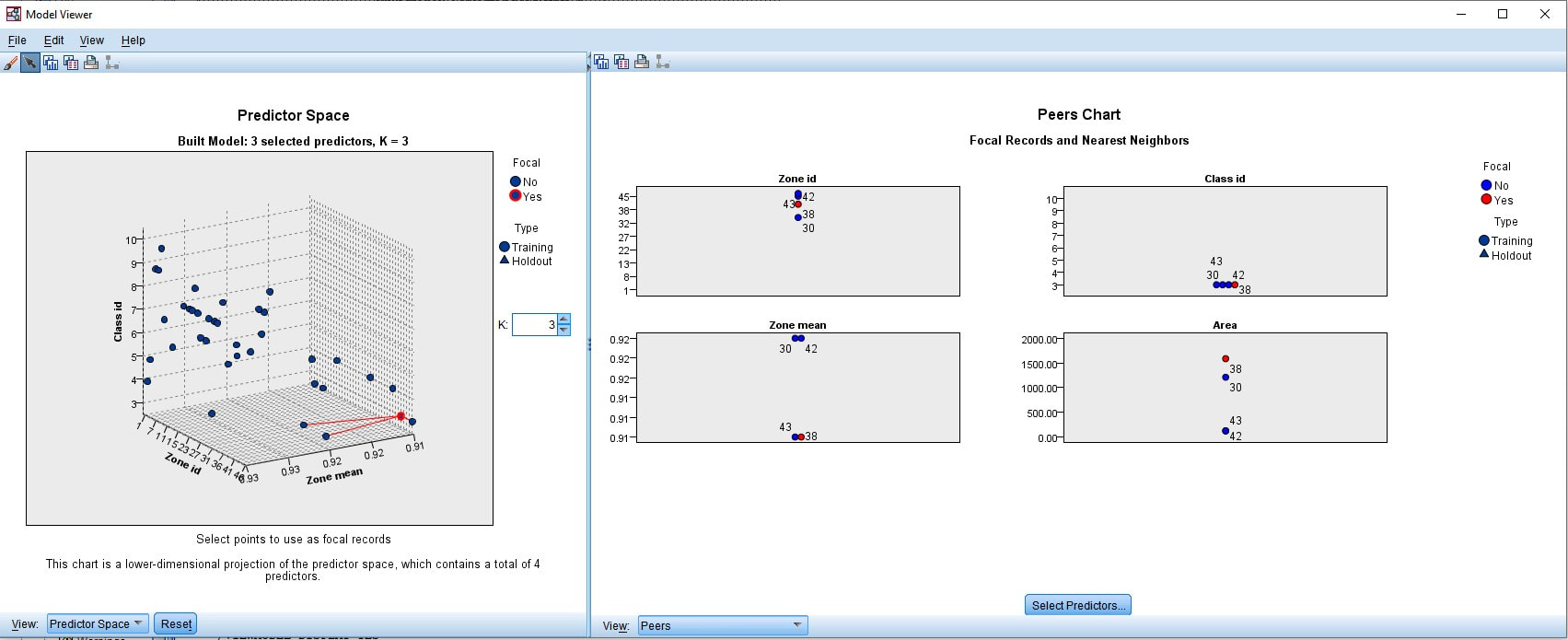
Figure 4. Presentation of the Predictor Space and Peers Chat with focal records and nearest neighbours for Zone id 38 from for table with statics data for 47 zones of forest area #1 (NDVI) from IBM SPSS Statistics.
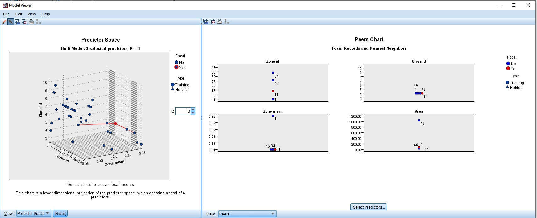
Figure 5. Presentation of the predictor space and peers chat with focal records and nearest neighbours for Zone id 11 from for table with statics data for 47 zones of forest area #1 (NDVI) from IBM SPSS Statistics.
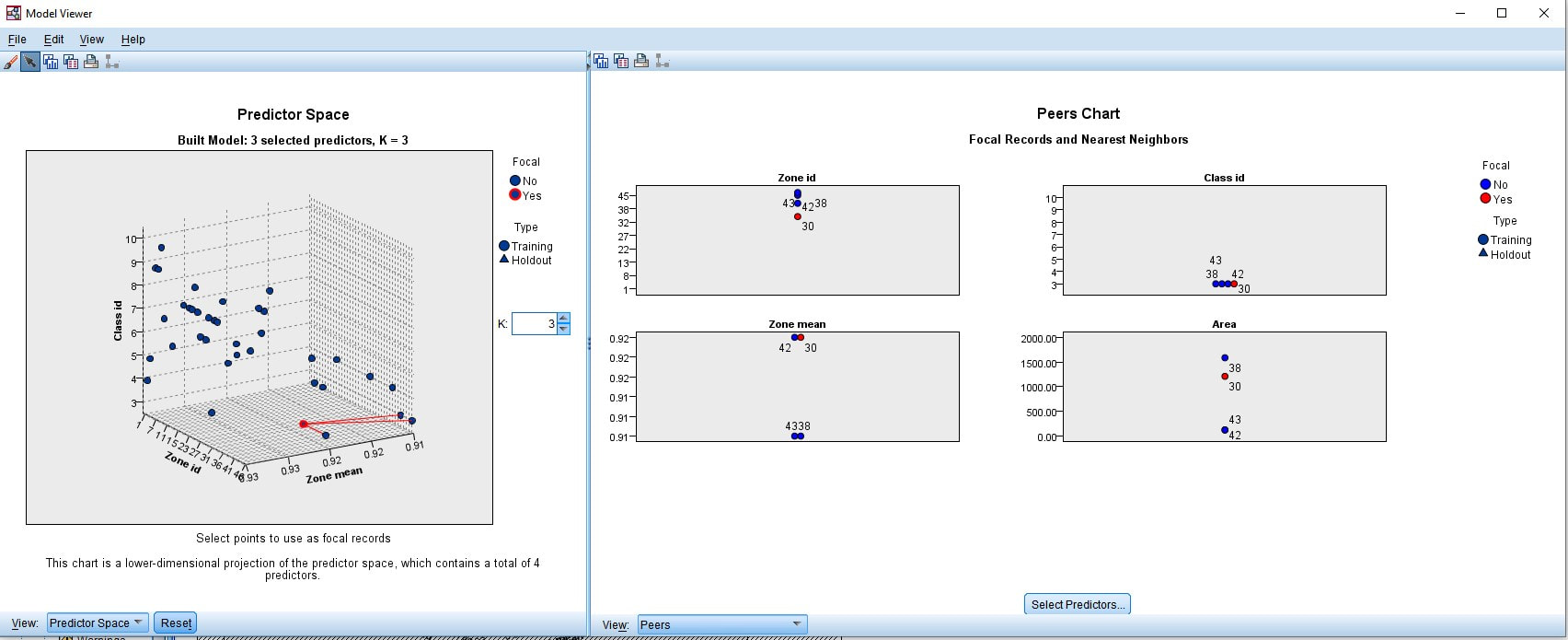
Figure 6. Presentation of the predictor space and peers chat with focal records and nearest neighbours for Zone id 30 from for table with statics data for 47 zones of forest area #1 (NDVI) from IBM SPSS Statistics.
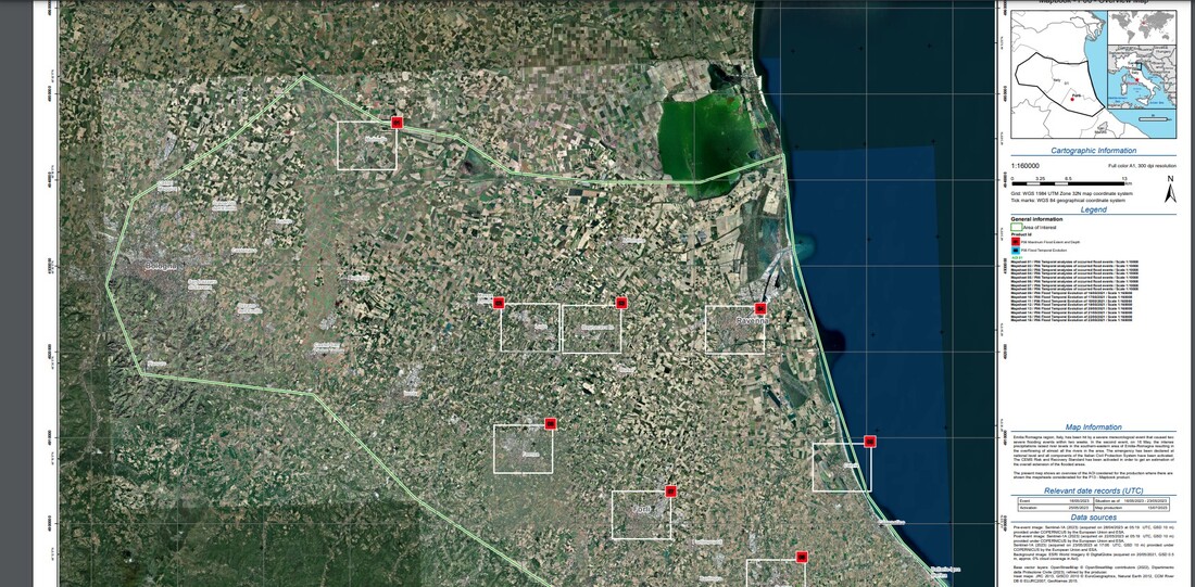
Figure 7. Presentation of the predictor space and peers chat with focal records and nearest neighbours for Zone id 13 from for table with statics data for 47 zones of forest area #1 (NDVI) from IBM SPSS Statistics.
Conclusions
Results of GIS/attribute data analysis using GIS mapping software and statistical software as IBM SPSS Statistics presented distance estimation between different statistics data for NDVI. The main goal is to conduct an analysis for NDVI, NDWI and SAVI with the addition of statistics data Zone Max, Zone min, P10, P 90 from the table #1 with statics data for 47 zones.
2. Carrying out clustering analysis with classification by zones according to clusters/classes to obtain statistics data (ESA SNAP).
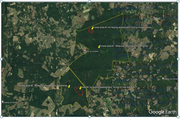
Figure 1. Location of the forest area #1 and forest area #2.
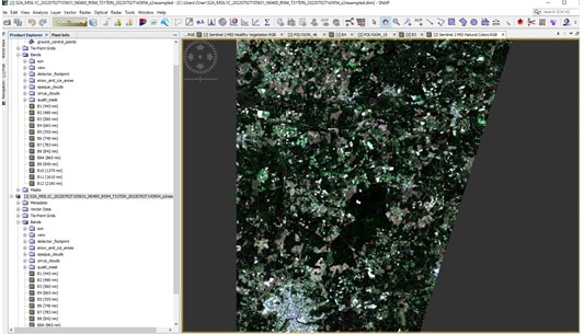
Figure 2. Location of forest area #1 in local communities in France.
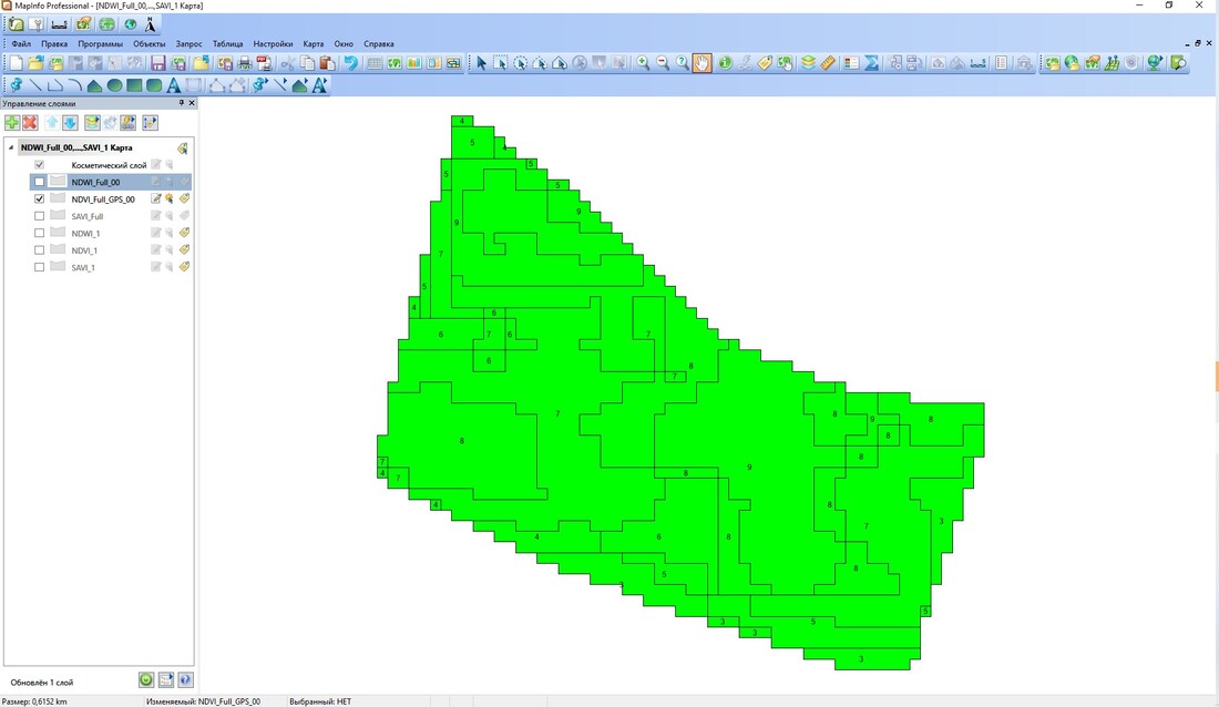
Figure 3. General preliminary analysis of attributive GIS data by NDVI, to identify sites with potential for tree drying and detection probability by MCI Natural Collors RGB.
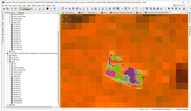
Figure 4. General preliminary analysis of attributive GIS data by NDVI, to identify sites with potential for tree drying and detection probability by MCI Land / Water RGB.
1. Perform remote sensing by used to three vegetation indexes; NDVI, NDWI and SAVI (EO Copernicus, ESA SNAP and EOS)
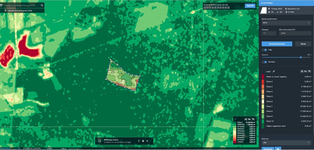
Figure 1. Analysis with clustering and classification with statisticals data NDVI
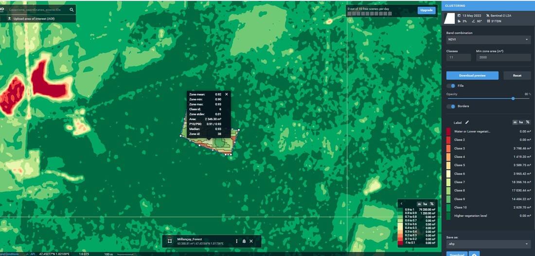
Figure 2. General preliminary analysis with clustering and classification to identify sites with high potential for tree drying and low detection probability by NDVI
Figure 3. Analysis after clustering and classification with NDVI statistical data for ZONE id =38, which is part of class 6.
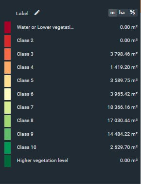
Figure 4. Figure 6.2 Map legend for class 6 for NDVI to which ZONE id =38 is included.
3. Transferring statistics data to GIS/attribute data (Map Info/Arc Gis online).
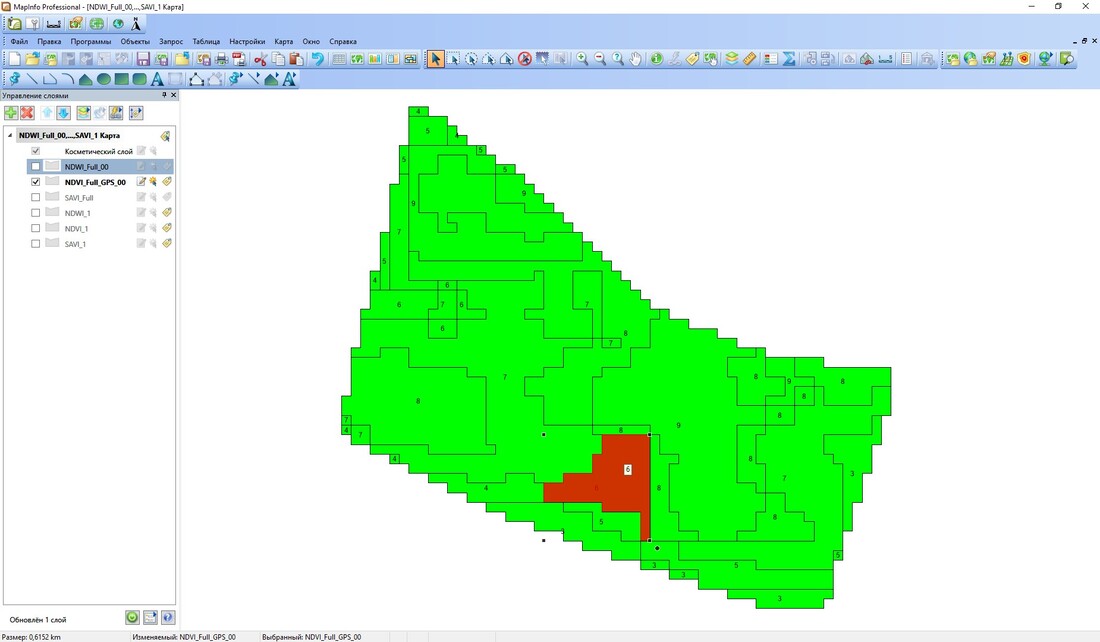
Figure 1. GIS map analysis after clustering and classification of testing forest area #1 by NDVI and statistics data.
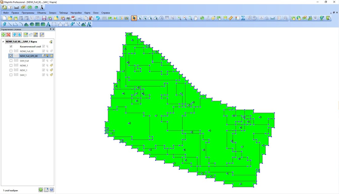
Figure 2. Coordinates of centroids of zones and their boundaries of NDVI for statistical analysis in SPSS Statistics.
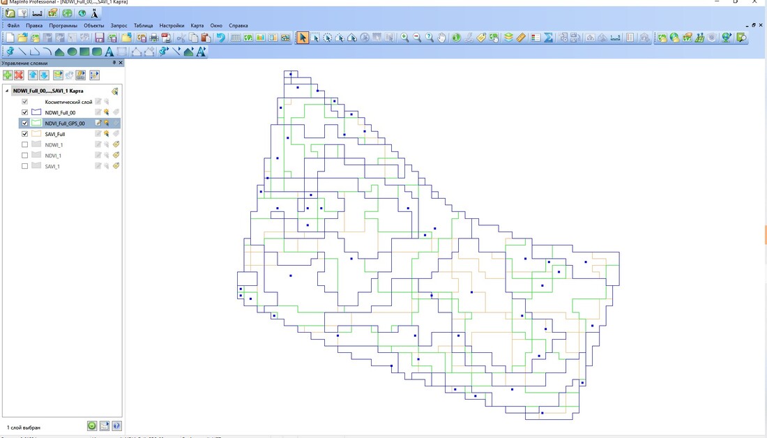
Figure 3. The result of overlay of clusters/zones of 3 VI with GIS/attribute data after clustering and classification in Map Info. The following clusters/zones are presented with colour development as indicated: 1. NDVI zones - green lines 2.) SAVI zones - orange lines); 3.) NDWI zones - blue lines).
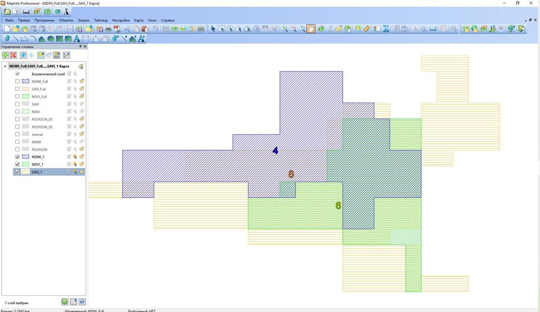
Figure 4. The result of overlay of 1 cluster/zone from 3 VI with GIS/attribute data after clustering and classification in Map Info. The following clusters/zones are presented: zone NDVI #6, zone SAVI #8, zone NDWI #4.
